Authors:

One Cindie Mogapi, Aditie Beura, Angel Khurana, Sharvi Makhija, Saanvi Vij, Suribhi Yadav, Geeta Pandey, Pranay Tripathi

ABSTRACT

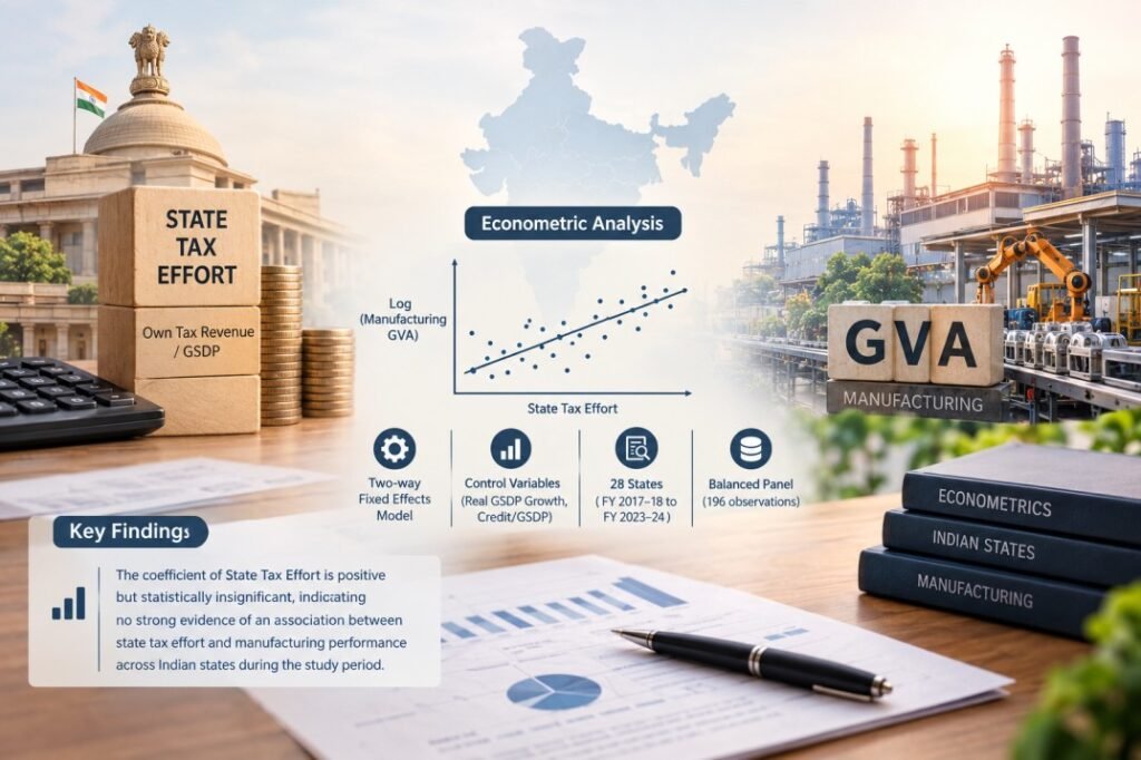
Manufacturing is important to India’s development because it contributes to output, employment, investment, and exports. In the post-GST period, it is relevant to examine whether differences in states’ own tax mobilization are associated with differences in manufacturing performance. This study analyses 28 Indian states from FY 2017–18 to FY 2023–24 using a balanced panel of 196 state-year observations. Manufacturing performance is measured by the logarithm of real Manufacturing Gross Value Added (GVA), while State Tax Effort is measured as Own Tax Revenue relative to Gross State Domestic Product (GSDP). Real GSDP growth and Credit/GSDP are included as control variables. A two-way fixed-effects regression model is used to account for state-specific characteristics and common year effects. The estimated coefficient of State Tax Effort is positive (0.910), but statistically insignificant (p = 0.703). The result remains statistically insignificant when lagged State Tax Effort is used and when the COVID-19 period is excluded. The study therefore finds insufficient statistical evidence of a significant association between State Tax Effort and manufacturing performance across Indian states during the study period.

Keywords:

State Tax Effort; Manufacturing GVA; Own Tax Revenue; GSDP; GST; Indian States; Two-Way Fixed Effects; Panel Data.

INTRODUCTION

Manufacturing plays an important role in developing the economy by contributing to production, employment, investment, exports, and ultimately economic growth. To develop the economy, especially in India, strengthening the manufacturing sector has been a vital effort to improve productive capacity and boost competitiveness. Still, the manufacturing sector in India has encountered numerous difficulties, including access to finance, skilled labor, technology, as well as differences in infrastructure and the broader business environment. These difficulties have increased the importance of policies aimed at creating conditions that can support sustained manufacturing growth.

Based on this, the Make in India initiative was launched by the Government of India in September 2014, with the mandate of strengthening domestic manufacturing, attracting investment, and encouraging foreign direct investment (FDI). These efforts were intended to create employment opportunities and improve India’s position in the global economy. Through this initiative, manufacturing was placed at the center of India’s development strategy, seeking to build a supportive environment for investors and businesses. However, the success of these goals depends on investment promotion policies, as well as the wider economic and institutional environment in which firms operate.

Another important part of this environment is taxation. Taxes provide the government with revenue, which is needed to finance public expenditure and development. However, the level and structure of taxation can influence business decisions, investment, and economic activity. A more predictable and efficient tax system may improve the conditions for investment and production, while a complex tax system or higher state tax effort may be associated with higher costs of operating a business. Therefore, it is important to consider tax policy when examining the factors that may be associated with manufacturing performance across different regions of India.

India experienced a major tax reform in an effort to simplify taxation, strengthen revenue collection, improve compliance, and create a more efficient tax system. In 2017, India introduced the Goods and Services Tax (GST), which brought a significant change in the country’s indirect tax structure by replacing multiple indirect taxes with a more unified system. In addition to GST, modifications to corporate taxes and other fiscal adjustments have reshaped the economic environment for Indian companies. Consequently, researchers have shown substantial interest in analyzing how these policies affect corporate investments, commercial operations, and overall economic growth.

Although policy initiatives strongly favor industrial growth, the relationship between taxation and manufacturing output remains uncertain without further empirical scrutiny. Because both manufacturing performance and state tax effort vary across states, these differences may reflect deeper regional economic disparities. Current academic scholarship covers India’s tax reforms and foreign investment broadly; however, few studies use post-GST panel data to examine the association between state tax effort and state-level manufacturing performance. Bridging this gap is important for examining whether state-level tax effort is associated with regional manufacturing performance.

This study examines the relationship between state-level tax effort and manufacturing performance across 28 Indian states during the period FY 2017–18 to FY 2023–24. Using secondary data from the Reserve Bank of India, the study measures manufacturing performance using the logarithm of real Manufacturing Gross Value Added (GVA) and state tax effort using Own Tax Revenue as a proportion of Gross State Domestic Product (GSDP). Real GSDP growth and bank credit relative to GSDP are included as control variables. A two-way fixed-effects panel regression is employed to account for both state-specific characteristics and year-specific factors. By focusing on the post-GST period, the study provides empirical evidence on the relationship between state-level tax effort and manufacturing performance across Indian states. Make in India provides the broader policy context for this study; the analysis does not evaluate the causal effect of Make in India itself.

LITERATURE REVIEW

1. Taxation, State Tax Effort and Manufacturing Performance

The relationship between taxation and economic activity is theoretically ambiguous. Taxation can influence private-sector decisions by affecting the resources available to firms for investment, expansion and production. At the same time, taxation constitutes an important source of government revenue and therefore contributes to the fiscal capacity required to provide public infrastructure, public services and other productive inputs. The relationship between tax mobilization and manufacturing performance consequently cannot be assumed to operate in only one direction.

The literature on India’s tax system has traditionally focused on the efficiency, structure and administration of taxation. Rao and Rao (2009) identify the complexity and structural weaknesses of India’s tax system as important reasons for reform, arguing for a system that is more efficient, broad-based and conducive to economic development. Rao and Kumar (2018) similarly examine tax policy in the context of accelerated development and emphasize the importance of balancing revenue mobilization with the need to minimize distortions to economic activity. These studies establish that the significance of taxation extends beyond the amount of revenue collected: the structure and administration of taxation can also influence the economic environment in which firms operate.

Thomas et al. (2017) provide a more direct connection between taxation and investment. Their analysis of taxation and investment in India highlights effective tax rates, the breadth of the tax base and uncertainty in the tax system as factors relevant to investment decisions. This suggests that taxation may affect economic activity through a cost channel, whereby higher or less predictable taxation can influence the incentives facing private investors.

However, the fiscal-capacity perspective provides an important counterargument. Tax revenue allows governments to finance expenditure that can create conditions favorable to private economic activity. The Reserve Bank of India’s State Finances: A Study of Budgets places considerable emphasis on the revenue dynamics and fiscal capacity of Indian states and highlights the importance of strengthening state finances while maintaining growth-enhancing public expenditure. Thus, higher tax mobilization need not necessarily imply a weaker environment for production. If additional revenue is translated into productive public expenditure, improved infrastructure or better public services, stronger state tax effort could coexist with stronger manufacturing performance.

This distinction is particularly important for the present study. The measure used here is not a tax rate imposed specifically on manufacturing firms. Instead, State Tax Effort (STE) is measured as own tax revenue relative to GSDP:

STEᵢₜ = (Own Tax Revenueᵢₜ / GSDPᵢₜ) × 100

This ratio captures the extent of own-source tax revenue mobilization relative to the size of the state economy. It should therefore be interpreted as an indicator of state fiscal effort, rather than as the effective tax burden faced by manufacturing firms. The distinction is important because a state with a higher tax-to-GSDP ratio is not necessarily imposing a higher effective tax rate on manufacturing enterprises.

Empirically, state tax effort also varies considerably across India. Recent work on Indian state finances documents substantial differences in own revenue and own-tax revenue relative to GSDP across states, suggesting meaningful cross-state variation in fiscal mobilization. Such variation provides a basis for examining whether differences in state tax effort are systematically associated with differences in manufacturing performance.

2. Taxation, Investment and Manufacturing: Indian Evidence

A second strand of literature examines the relationship between taxation and private investment, which provides a potential mechanism connecting state tax effort with manufacturing performance.

Singh (2016) examines India’s taxation environment in relation to foreign direct investment and argues that taxation forms an important component of the investment climate. Thomas et al. (2017) similarly highlight the relevance of taxation to investment decisions. These studies suggest that the tax environment can influence the attractiveness of investment by affecting expected returns, compliance costs and the predictability of the business environment.

More recent empirical studies provide evidence at the firm level. Sankarganesh and Shanmugam (2023) examine Indian manufacturing firms and find a negative relationship between effective corporate income taxation and investment. Their findings suggest that taxation can influence firms’ investment decisions, providing empirical support for the tax-cost channel. However, their measure of taxation relates to corporate taxation faced by firms and is therefore conceptually different from the state tax-effort measure employed in the present study.

Hussain (2023) provides further evidence using India’s 2019–20 corporate tax reform. Employing a difference-in-differences framework, the study finds a significant increase in investment among domestic manufacturing firms following the reduction in the corporate tax rate, with the response being stronger among larger firms. This provides evidence that a specific change in corporate taxation can influence manufacturing-firm investment.

These findings are relevant but do not directly answer the question examined in the present study. Both studies focus on firm-level corporate taxation, whereas the present analysis examines state-level own tax mobilization relative to GSDP. The distinction matters because state tax effort captures a broader fiscal environment rather than the effective tax rate faced by an individual manufacturing firm.

Moreover, increased investment does not necessarily imply an increase in manufacturing GVA at the state level. The transmission from taxation to manufacturing performance may depend on other conditions, including access to finance, infrastructure, skills, technology and the overall economic environment. The existing firm-level evidence therefore motivates the question of whether a similar relationship is observable at the state level, while also indicating why the relationship may not be one-to-one.

3. State Fiscal Capacity and Manufacturing

The state-level dimension of taxation is particularly important in India because state governments play a substantial role in the provision of infrastructure and public services that influence the environment in which economic activity takes place.

The literature on state finances increasingly treats revenue mobilization as an element of fiscal capacity rather than simply as a measure of taxation. The RBI’s State Finances: A Study of Budgets examines the revenue dynamics and fiscal capacity of Indian states and emphasizes the importance of strengthening state finances while maintaining expenditure that supports growth. This perspective provides a basis for considering state tax effort as potentially relevant to manufacturing through the expenditure and public-input channel.

Rao and Kumar (2018) similarly emphasize the broader developmental role of tax policy. Their work suggests that tax policy must be considered in relation to the government’s capacity to finance development while maintaining an environment conducive to economic activity.

The relationship between fiscal capacity and manufacturing is therefore potentially different from the relationship between firm-level tax rates and investment. A higher state tax-effort ratio may indicate greater extraction of resources from the private sector, but it may also indicate stronger revenue mobilization and therefore greater fiscal capacity. The empirical relationship depends partly on what the state does with the revenue it mobilizes.

This is particularly relevant to manufacturing because manufacturing activity is sensitive to infrastructure, logistics, electricity, transport networks, skills and other public inputs. Deodhar (2015), in discussing Make in India, argues that investment promotion alone is insufficient for sustained manufacturing growth and identifies infrastructure, labor regulations, land, technology and the broader business environment as important constraints. Kadekodi (2018) similarly emphasizes infrastructure, productivity, skilled labor, finance and technology as important determinants of manufacturing performance.

Consequently, the literature suggests that the relationship between state tax effort and manufacturing performance may operate through competing mechanisms. Higher state tax effort may represent a greater fiscal cost to the private sector, but it may simultaneously strengthen the state’s capacity to provide the public inputs necessary for manufacturing.

4.Financial Conditions and Manufacturing: The Credit Channel

The availability of finance represents another important factor in manufacturing performance. Manufacturing firms require working capital as well as longer-term financing for investment in machinery, technology, capacity expansion and other productive assets. Consequently, differences in credit availability across states may influence manufacturing activity independently of taxation.

The inclusion of credit conditions is therefore important when examining the relationship between state tax effort and manufacturing performance. If states with stronger manufacturing sectors also have deeper financial systems and greater access to formal credit, a simple relationship between state tax effort and manufacturing could partly reflect differences in financial conditions rather than taxation itself.

For this reason, the present study incorporates Credit/GSDP as a control variable. The ratio provides an indicator of the scale of bank credit relative to the size of the state economy and captures the broader financing environment within which firms operate.

The importance of financing conditions is also consistent with the broader Make in India literature. Kadekodi (2018) identifies access to finance as one of the factors influencing manufacturing performance, while Deodhar (2015) emphasises that manufacturing competitiveness depends on a wider ecosystem rather than on investment promotion alone.

The credit channel therefore serves two purposes in the present analysis. First, it represents an economically relevant determinant of manufacturing performance. Second, controlling for Credit/GSDP reduces the possibility that the estimated association between state tax effort and manufacturing GVA simply reflects differences in financial development across states.

5. Economic Conditions and Manufacturing Performance

Manufacturing performance is also closely connected to the broader economic conditions prevailing within a state. Periods of stronger economic growth may generate greater demand for manufactured goods, increase private investment and expand the productive base. At the same time, stronger economic activity can increase tax collections. This creates a potential relationship between state tax effort and manufacturing that may arise partly because both variables respond to overall economic conditions.

The inclusion of GSDP growth therefore provides an important control in the empirical framework. By accounting for broader state-level economic growth, the analysis attempts to distinguish the relationship between state tax effort and manufacturing performance from the general economic conditions prevailing in a state.

Official data also demonstrate substantial variation in industrial and manufacturing structures across Indian states. The Economic Survey notes that manufacturing constitutes a significant component of state industrial activity, while the degree of industrial dependence differs considerably across states. This heterogeneity reinforces the importance of examining the relationship using state-level rather than only aggregate national data.

The use of state and year fixed effects further strengthens this approach. State fixed effects account for time-invariant characteristics that may differ across states, while year fixed effects capture common shocks affecting states in a particular year. Such controls are especially relevant for a period that includes major economy-wide developments and the COVID-19 disruption.

6. Make in India as the Policy Context

The Make in India initiative, launched in 2014, provides the broader policy context within which the present study examines manufacturing performance. The initiative sought to strengthen domestic manufacturing, attract investment and improve India’s competitiveness. However, the literature on Make in India consistently indicates that manufacturing performance depends on more than investment promotion alone.

Deodhar (2015) argues that the success of Make in India requires improvements in infrastructure, labour regulations, land access, technology and the broader business environment. Kadekodi (2018) similarly identifies productivity, infrastructure, skilled labour, finance and technology as important determinants of manufacturing performance. Som (2018) further highlights the distinction between an improved investment environment and actual manufacturing outcomes, suggesting that stronger investment conditions do not automatically translate into proportional increases in manufacturing value added.

Taxation forms part of this wider policy environment. GST represented a major restructuring of India’s indirect tax system, with the literature highlighting potential improvements in tax uniformity, logistics and the functioning of the domestic market. Ojha and Vrat (2019), for example, examine the implications of GST for Make in India through a system-dynamics framework and identify several channels through which tax reform could influence manufacturing.

However, the present study does not estimate the effect of Make in India itself. Make in India is treated as the policy context rather than as an explanatory variable in the empirical model. The study instead asks whether differences in state-level tax effort are associated with differences in manufacturing performance during the period in which the Make in India policy framework was being pursued.

This distinction is important because the empirical model contains no direct measure of Make in India. It would therefore be inappropriate to interpret the estimated coefficient on state tax effort as the effect of Make in India or to claim that the study establishes the impact of the initiative.

7. Synthesis of the Literature

The literature reveals that taxation and manufacturing can be connected through at least two competing mechanisms.

The first is the tax-cost channel. Higher taxation or a less favourable tax environment may reduce the resources available to firms and affect investment incentives. Evidence from Indian manufacturing firms supports the relevance of this channel: Sankarganesh and Shanmugam (2023) find a negative relationship between effective corporate taxation and investment, while Hussain (2023) finds a positive investment response following the 2019–20 corporate tax reduction.

The second is the fiscal-capacity channel. Greater tax mobilisation can increase the resources available to state governments and potentially support infrastructure, public services and other productive inputs. RBI’s work on state finances explicitly frames own-revenue mobilisation within the broader question of state fiscal capacity and the ability of states to undertake growth-enhancing expenditure.

These mechanisms imply that the relationship between state tax effort and manufacturing performance is theoretically ambiguous. A higher own-tax-revenue-to-GSDP ratio cannot automatically be interpreted as either a constraint on manufacturing or a source of manufacturing growth.

The literature also indicates that manufacturing performance depends on several factors beyond taxation. Infrastructure, skills, technology, finance and the broader economic environment have repeatedly been identified as important determinants of manufacturing performance (Deodhar, 2015; Kadekodi, 2018). This provides a rationale for incorporating Credit/GSDP and GSDP growth as controls in the empirical model.

Methodologically, an important distinction also emerges. A considerable part of the Indian literature examines taxation and investment at the firm or national level, while studies of state fiscal capacity generally focus on revenue mobilisation and state finances. Comparatively less attention has been given to whether differences in state-level tax effort are associated with differences in manufacturing GVA across Indian states after accounting for unobserved state characteristics, common time effects and broader economic and financial conditions.

8. Research Gap and Research Question 

The existing literature provides substantial evidence on taxation, investment, state fiscal capacity and manufacturing performance, but these relationships have largely been examined through separate strands of research.

First, existing studies on taxation and investment primarily examine firm-level corporate taxation rather than state-level own tax mobilisation. Consequently, their findings cannot be directly interpreted as evidence on the relationship between a state’s own tax effort and its manufacturing performance.

Second, the literature on state finances establishes substantial differences in tax mobilisation and fiscal capacity across Indian states, but comparatively less empirical work directly connects these differences to manufacturing GVA. RBI’s state-finance literature provides extensive evidence on state revenue mobilisation and fiscal capacity, but its principal focus is on the fiscal position and finances of state governments rather than on the state tax effort–manufacturing relationship.

Third, the Make in India literature emphasises the importance of manufacturing and identifies taxation, infrastructure, finance, skills and technology as components of the broader business environment. However, Make in India is generally studied as a policy initiative rather than through a state-level empirical specification linking tax mobilisation to manufacturing performance.

Finally, much of the existing literature is descriptive, conceptual or focused on specific reforms. While firm-level econometric studies such as Sankarganesh and Shanmugam (2023) and Hussain (2023) provide stronger empirical evidence, there remains limited evidence examining the relationship between state tax effort and manufacturing performance across Indian states within a panel framework.

Research Gap:

Limited empirical evidence examines the association between state-level tax effort, measured by own tax revenue relative to GSDP, and manufacturing performance across Indian states using a two-way fixed-effects panel framework.

The present study addresses this gap by examining whether state tax effort is significantly associated with manufacturing performance across 28 Indian states during FY 2017–18 to FY 2023–24, while controlling for GSDP growth, Credit/GSDP, state-specific effects and year-specific effects.

Research Question :

Is state tax effort, measured by own tax revenue relative to GSDP, significantly associated with manufacturing performance across Indian states during FY 2017–18 to FY 2023–24, after controlling for GSDP growth, Credit/GSDP, state fixed effects and year fixed effects?

This formulation keeps the research question strictly aligned with the empirical model. It does not claim to estimate the causal effect of taxation, GST or Make in India, but tests whether a statistically significant association exists between state tax effort and manufacturing performance.

Null Hypothesis (H0) : β₁ = 0:

There is no statistically significant association between state tax effort (measured as own tax revenue relative to GSDP) and manufacturing performance (measured as the natural logarithm of real manufacturing GVA) across Indian states during the period FY 2017–18 to FY 2023–24.

RESEARCH METHODOLOGY

1. Research Design

For the empirical investigation of this study, a quantitative empirical research design is  adopted. It aims at investigating the relationship between state tax effort and manufacturing performance in India’s states. The period under examination is the financial years of 2017-18 till 2023-24. For this purpose, panel data of the states is used as the post-GST period. Use of panel data is made here because it makes use of the observations of different years and states, thus change in manufacturing performance can be considered in different states.

The fixed effect regression is used in which there are state fixed effects and year fixed effects. Use of state fixed effects takes into consideration the characteristics of the state which persists over time, whereas year fixed effects take into account those changes which happened in a particular year. The main objective of the analysis is to investigate whether the difference in the state level tax effort affects manufacturing performance.

Justification of Methodology

The methodology is chosen to match the research question: how State Tax Effort is related to manufacturing performance across Indian states after GST. Because the data cover multiple states over several years, a panel-data framework is the natural choice. The final sample is a balanced panel of 196 state-year observations for 28 states from FY 2017–18 to FY 2023–24. This structure lets the analysis use both cross-state differences and within-state changes over time.

A two-way fixed-effects specification is used for two main reasons. Firstly, states differ in ways that are hard to measure directly—such as historical industrial structure, institutional quality, geography, and long-run policy environments. State fixed effects absorb these time-invariant, state-specific factors. Secondly, all states are exposed to common shocks in a given year (for example, national business-cycle conditions, commodity-price movements, or economy-wide policy changes). Year fixed effects capture these common time effects. Together, state and year fixed effects provide a cleaner setting to study the link between State Tax Effort and manufacturing performance than a simple pooled regression.

The dependent variable is the natural logarithm of real Manufacturing Gross Value Added (GVA). Using the log of real GVA helps capture manufacturing performance while limiting the influence of sheer size differences across states. State Tax Effort is defined as a state’s Own Tax Revenue divided by its GSDP. This is intended as a measure of fiscal effort—how much revenue a state mobilises from its own sources relative to the size of its economy—rather than as a direct measure of the state tax effort on manufacturing firms.

Real GSDP growth and the ratio of credit to GSDP are included as controls. Manufacturing outcomes are likely to move with overall state economic conditions and with the availability of finance. Adding these controls helps separate the association between State Tax Effort and manufacturing performance from broader growth dynamics and credit conditions.

The study period, FY 2017–18 to FY 2023–24, corresponds to the post-GST era and offers a consistent window to examine State Tax Effort and manufacturing performance after the reform. The analysis does not try to identify the causal impact of GST or of initiatives such as Make in India; it simply uses this period as a coherent post-reform timeframe.

In sum, the empirical design aims to test whether State Tax Effort is statistically associated with manufacturing performance after controlling for state-specific factors, year-specific shocks, overall economic growth, and credit availability. Given the possibility of unobserved time-varying influences on manufacturing, the results are best interpreted as associations, not causal effects.

Nature of Research

The research is quantitative and empirical in nature, which is completely based on secondary data. The research is based on state-level data from FY 2017–18 to FY 2023–24 in order to find out the relationship between state tax effort and manufacturing performance in India. The post-GST era is the focus of this research since GST is one of the significant parts of the tax reform in this research.

The publicly available data from the Reserve Bank of India (RBI) is used in this research. The data is arranged into the state-year data format to create panel data. It means that the difference across the states and the difference through the year for each state can be analysed through this data. The research is based on statistics and econometrics, not surveys and interviews.

2. Sample & its Technique

In this research paper, panel data from Indian states is utilized for the financial years 2017-18 to 2023-24. This dataset comprises 28 states over a period of 7 financial years, which provides a balanced panel of 196 observations of the states-year wise. In the dataset, all 28 states have been included without limiting the sample to the major manufacturing states in India to account for the variance in manufacturing among Indian states.

Data Collection Tool

The study is based on secondary data collected from official publications and statistical databases of the Reserve Bank of India (RBI). The analysis covers the period from FY 2017–18 to FY 2023–24 and uses state-level observations to construct a panel dataset for the post-GST period. The relevant data were identified and compiled from RBI sources based on their relevance to the variables specified in the empirical model.

The principal source was the RBI Handbook of Statistics on Indian States, which provided state-level information on GSDP, Manufacturing GVA and Own Tax Revenue. The RBI State Finances publications were additionally consulted to cross-check the Own Tax Revenue figures. Information on outstanding bank credit was obtained from the RBI’s Basic Statistical Returns (BSR-1), which provides state-wise banking data. For consistency with the financial-year framework of the study, the BSR-1 observations were aligned with the corresponding March values; for instance, FY 2017–18 was matched with March 2018 and FY 2023–24 with March 2024.

The collected data were then used to construct the analytical variables required for the empirical model. Specifically, state tax effort was derived from Own Tax Revenue relative to GSDP, bank credit was expressed relative to GSDP, and Manufacturing GVA was transformed into its natural logarithm.

Prior to estimation, the compiled data were checked for unit consistency, constant-price definitions, missing observations and potential outliers. These checks were undertaken to ensure that the indicators were comparable across states and years before their inclusion in the panel regression.

3. Variables Used

The empirical analysis examines the relationship between state-level tax effort and manufacturing performance. The dependent variable, principal explanatory variable, and control variables are defined and operationalised as follows.

Manufacturing GVA

Real manufacturing GVA is used as the dependent variable and represents manufacturing performance at the state level. It is measured using constant-price GVA which allows changes in manufacturing activity to be examined in real terms rather than being influenced by changes in prices. Manufacturing GVA is expressed in logarithmic form in the empirical model, which also helps reduce differences in scale across states.

State Tax Effort

The main explanatory variable is the state’s own tax revenue relative to its GSDP, calculated as:

State Tax Effortᵢₜ = (Own Tax Revenueᵢₜ / GSDPᵢₜ) × 100

where i represents the state and t represents the year.

Using a ratio rather than absolute tax revenue makes the measure more comparable across states with substantially different economic sizes. The measure captures the state’s own tax collections relative to the size of its economy and is therefore used as a proxy for state-level tax effort. It should be noted that it does not represent the effective tax rate faced by individual manufacturing firms.

Real GSDP growth

Real GSDP growth is measured as the annual percentage growth in real GSDP and is included as a control variable for broader economic conditions within a state. Manufacturing activity may expand alongside overall economic activity, while tax collections may also change as the state economy grows. Including GSDP growth therefore helps distinguish the relationship between state tax effort and manufacturing performance from changes associated with the general economic cycle.

Bank credit relative to GSDP

Bank credit relative to GSDP is included to capture differences in financing conditions across states. The variable is calculated as outstanding bank credit as a proportion of GSDP:

Credit/GSDP_it = (Outstanding Bank Credit_it / GSDP_it ) × 100

where i represents the state and t represents the year.

Access to credit can influence the ability of manufacturing firms to finance working capital, investment and expansion. Controlling for credit availability therefore helps account for differences in financial conditions that may otherwise be reflected in the estimated relationship between taxation and manufacturing performance. The relationship between tax burden and manufacturing performance is estimated using a panel-data fixed effects regression.

The model is expressed as:

ln(MFGVAᵢₜ) = αᵢ + λₜ + β₁StateTaxEffortᵢₜ + β₂GSDPGrowthᵢₜ + β₃Credit/GSDPᵢₜ + εᵢₜ

where,

State Tax Effortᵢₜ = (Own Tax Revenueᵢₜ / GSDPᵢₜ) × 100

Credit/GSDP_it = (Outstanding Bank Credit_it / GSDP_it ) × 100

Real GSDP Growth Rate_it = [(Real GSDP_it – Real GSDP_i,t-1) / Real GSDP_i,t-1 ] × 100 

The model incorporates state fixed effects and year fixed effects. State fixed effects account for persistent characteristics of individual states, such as historical industrialisation, geography and established industrial structures, while year fixed effects account for shocks and conditions common across states in a given year. The standard errors are clustered at the state level.

4. Limitations of the model

The study has certain limitations that should be considered while interpreting its findings. First, the model does not establish a causal relationship between state tax effort and manufacturing performance. Although state and year fixed effects account for differences between states and common changes across years, there may still be other factors that affect both taxation and manufacturing. There may also be reverse causality, as changes in manufacturing activity could themselves affect tax collections. Therefore, the results should be understood as showing an association between the variables, rather than proving that changes in state tax effort directly cause changes in manufacturing performance.

Second, state tax effort is measured using Own Tax Revenue as a percentage of GSDP. This provides a useful measure for comparing states of different economic sizes, but it does not directly measure the state tax effort faced by individual manufacturing firms. Differences in the types of taxes collected by states and who ultimately bears these taxes may therefore not be fully captured by the measure.

Third, the study covers a relatively short period from FY 2017–18 to FY 2023–24. This limits the number of years available for observing changes in taxation and manufacturing performance and makes it difficult to assess longer-term trends.

The study also depends on secondary data from RBI sources. Differences in data availability, definitions, or reporting across states and years may affect how comparable the observations are. The data were checked for consistency in units and price definitions, as well as for missing values and potential outliers, but some limitations of the original data may still remain.

Finally, the study includes FY 2020–21, which was affected by the COVID-19 pandemic. The sharp changes in economic activity during this period may have influenced both manufacturing and tax collections in ways that are different from normal economic conditions. This may affect the estimated relationship, which is why the study also considers a robustness check that excludes the COVID-affected period.

DATA ANALYSIS

The analysis examines the relationship between state-level tax burden and manufacturing performance across Indian states. The study uses secondary data from the Reserve Bank of India (RBI) for 28 Indian states over the period 2017–2024. The data is structured as panel data, with observations recorded for individual states across different years.

Dependent Variable: Manufacturing performance = Ln(Manufacturing Gross Value Added)

Main Independent Variable: State Tax Effortᵢₜ = (Own Tax Revenueᵢₜ / GSDPᵢₜ) × 100

Control Variables:

Credit/GSDP_it = (Outstanding Bank Credit_it / GSDP_it ) × 100

Real GSDP Growth Rate_it = [(Real GSDP_it – Real GSDP_i,t-1) / Real GSDP_i,t-1 ] × 100 

Manufacturing performance is measured using the logarithm of Manufacturing Gross Value Added (GVA). The main explanatory variable is State tax effort. GSDP growth rate (measured as the annual percentage growth in real GSDP) and Credit/GSDP are included as control variables. The purpose of the analysis is to examine whether differences in state tax effort are associated with differences in manufacturing performance, after accounting for other economic and financial factors. The analysis begins with an overview of the sample and descriptive statistics, followed by correlation and regression analysis.

1.Data Overview and Sample Profile

The dataset covers 28 Indian states over FY 2017–18 to FY 2023–24, giving 196 state-year observations for the balanced panel. The baseline regression uses 196 observations, with the final number of observations determined by the availability of data for the variables included in the model. The sample therefore represents Indian states observed over multiple years and captures variation in their economic, fiscal and financial conditions.

Four main variables are used in the analysis. Manufacturing GVA (log) is used as the measure of manufacturing performance. State tax effort measures own tax revenue relative to GSDP. GSDP growth represents the annual growth of the state economy, while Credit/GSDP measures bank credit relative to GSDP.

The variables show substantial variation across the observations. Manufacturing GVA (log) ranges from 8.655 to 17.600, while tax burden ranges from 3.945% to 14.880%. GSDP growth ranges from −12.100% to 16.420%, showing differences in economic growth across states and years. Credit/GSDP has the widest range, from 10.779% to 136.854%. These descriptive statistics provide an initial picture of the differences present in the sample before the relationships between the variables are examined further.

2. Descriptive Statistics

Table 1 : Descriptive Statistics

Variable	Mean	SD	Min	Median	Max
Ln Manufacturing GVA	14.765	2.294	8.655	15.56	17.60
State Tax Effort (%)	8.760	2.168	3.945	8.793	14.88
GSDP growth (%)	5.323	5.102	-12.10	6.310	16.420
Credit/GSDP (%)	46.10	23.62	10.77	39.98	136.85

Source: Author’s calculation based on secondary data.

Manufacturing GVA (log) distribution skews toward lower values which has mean of 14.765 and higher median of 15.563. The Descriptive statistics are unable to pinpoint the states or years causing this skew, this pattern is consistent with a state year exhibiting noticeably weaker manufacturing performance. The state tax effort ranges from 3.94% to 14.88% with an average of 8.76% which is close to the median of 8.79%. The closeness of the mean and median suggests that the state tax effort distribution is relatively balanced around its central value, although there is meaningful variation across state-year observations. GSDP growth is 5.32% on an average but its standard deviation is 5.102 which is almost as high as the mean. Growth by 6.31% points, from a contraction of -12.10% to an expansion of 16.42% the source of this contraction cannot be confirmed by descriptive data, it is consistent with significant volatility in state-level development, perhaps representing a severe downturn in at least one year. With a mean of 46.10% and a median of 39.98%, a difference of more than 6% points, credit/GSDP exhibits the largest dispersion of all variables. Over 126% points separate the values, which range from 10.77% to 136.85%. Although descriptive statistics by themselves are unable to identify the states or sources causing this dispersion, the pattern is consistent with a small number of financially deeper states moving the distribution upward.

3. Distribution and Group Comparison

To further examine the distribution of the key variables, the 196 state-year observations are divided into four equal-sized groups (quartiles) according to their tax burden. The first quartile (Q1) represents observations with the lowest tax burden, while the fourth quartile (Q4) represents observations with the highest state tax effort. Each quartile contains 49 state-year observations. The comparison provides a descriptive assessment of how manufacturing performance, GSDP growth and credit availability differ across observations with different levels of state tax effort. These group comparisons are descriptive and should not be interpreted as evidence of causality.

Table 2 : Group Comparison by State Tax Effort Quartile

State Tax-Effort Group	Observations	Mean Tax Burden (%)	Mean Log Manufacturing GVA	Mean GSDP Growth (%)	Mean Credit/GSDP (%)
Q1 – Lowest	49	6.03	12.89	5.99	26.48
Q2	49	8.15	14.9	3.41	41.72
Q3	49	9.3	15.55	5.11	53.41
Q4 – Highest	49	11.57	15.71	6.79	62.82

 

Source: Author’s calculation based on secondary data.

Note: The 196 state-year observations are divided into four equal-sized groups based on tax burden.

The quartile comparison shows a clear descriptive gradient in manufacturing performance across tax-burden groups. Mean tax burden increases from 6.03% in the lowest-tax-burden group (Q1) to 11.57% in the highest-tax-burden group (Q4). Over the same groups, mean log Manufacturing GVA rises from 12.89 in Q1 to 15.71 in Q4. Thus, state-year observations with higher tax burdens tend, on average, to be associated with higher levels of manufacturing GVA in the pooled sample.

A similar positive pattern is observed for Credit/GSDP. Mean Credit/GSDP increases from 26.48% in Q1 to 62.82% in Q4. This indicates that observations with higher tax burdens also tend to have greater bank credit relative to the size of their economies. The pattern is consistent with the positive association between tax burden and Credit/GSDP observed in the subsequent correlation analysis.

The pattern for GSDP growth is less uniform. Mean GSDP growth is 5.99% in Q1, declines to 3.41% in Q2, and then increases to 5.11% in Q3 and 6.79% in Q4. Hence, unlike manufacturing GVA and Credit/GSDP, economic growth does not exhibit a consistent monotonic relationship across the tax-burden quartiles.

Overall, the quartile analysis indicates that observations in the higher tax-burden groups tend to have higher average manufacturing GVA and greater credit availability than observations in the lower tax-burden groups. However, these differences may reflect underlying differences in economic structure, fiscal capacity, financial development and other state-level characteristics. Therefore, the quartile comparison is used only to describe the distributional patterns in the data. The subsequent correlation and fixed-effects analyses provide a more formal examination of the relationship between state tax effort and manufacturing performance.

4. Variable-wise Analysis

This section examines the association between each explanatory variable and the outcome variable, prior to the formal regression analysis. The purpose is to identify raw, bivariate patterns in the data i.e, associations that have not yet been adjusted for state and year fixed effects and for the influence of other explanatory variables. These patterns provide context for interpreting the fixed-effects results that follow but they should not themselves be read as evidence of a causal relationship.

Correlation Matrix

Table 3 presents the pairwise Pearson correlation coefficients between manufacturing GVA (in logarithmic form) and the three explanatory variables used in the empirical model i.e, tax burden, real GSDP growth, and credit relative to GSDP.

Table 3: Pairwise Correlation Matrix (N = 196 state-year observations)

	Manufacturing GVA	State Tax Effort	GSDP Growth	Credit/GSDP
Manufacturing GVA	1.00	0.48	0.01	0.56
State Tax Effort	0.48	1.00	0.13	0.58
GSDP Growth	0.01	0.13	1.00	-0.04
Credit/GSDP	0.56	0.58	-0.04	1.00

Source: Author’s calculation based on secondary data

Manufacturing GVA and tax burden show a moderate positive raw correlation (r = 0.48), indicating that state-years with a higher own-tax-revenue-to-GSDP ratio tend, on average, to also record higher manufacturing GVA. Manufacturing GVA and credit relative to GSDP show a similarly moderate, and marginally stronger, positive correlation (r = 0.56). Manufacturing GVA and GSDP growth show almost no linear association (r = 0.01), suggesting that year-on-year economic growth is not strongly related to the level of manufacturing GVA in this sample. Tax burden and Credit/GSDP are themselves moderately correlated (r = 0.58), which motivates the multicollinearity check reported separately.

It is important to note that these are simple bivariate correlations and do not account for state fixed effects, year fixed effects, or the joint influence of the other explanatory variables. A raw positive correlation between tax burden and manufacturing GVA does not, by itself, imply that a higher tax burden causes higher manufacturing output; states with historically stronger industrial bases may simply also have higher own-tax-revenue capacity. The fixed-effects regression in Section 5 under data analysis addresses this limitation by exploiting within-state variation while controlling for common year-specific shocks.

Scatter Diagram: Tax Burden and Manufacturing GVA

Figure 1 visualises the positive pooled association between tax burden and log manufacturing GVA reported in Table 3 (r = 0.484). The scatter shows considerable dispersion around the fitted linear trend, indicating that state-years with similar tax-burden levels can still have substantially different manufacturing GVA. This dispersion is consistent with the influence of other state-level factors and reinforces the need for the fixed-effects analysis that follows.

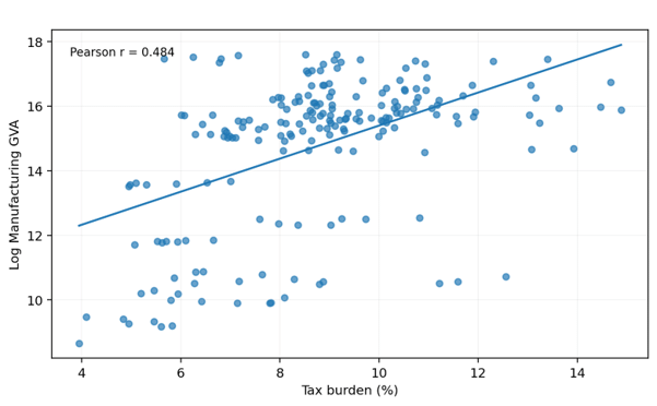
Figure 1. Relationship between Tax Burden and Manufacturing GVA

Note: Each point represents a state-year observation. The fitted line shows the unconditional linear trend. Tax burden is measured as own-tax-revenue-to-GSDP in percentage terms. Correlation is calculated using the project dataset (196 observations).

Credit Availability and Manufacturing GVA

Credit availability exhibits the strongest simple association with manufacturing GVA among the three explanatory variables. The Pearson correlation coefficient between Credit/GSDP and log manufacturing GVA is 0.561. This moderate positive relationship is consistent with the economic role of finance in supporting investment and working-capital requirements of manufacturing firms. Nevertheless, the descriptive relationship does not establish causality because higher manufacturing activity can itself be associated with greater demand for bank credit, while other state-level characteristics may influence both variables.

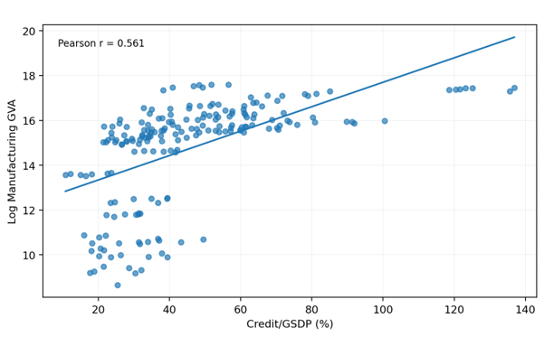
Figure 2. Relationship between Credit Availability and Manufacturing GVA

Note: Each point represents a state-year observation. Credit availability is measured as bank credit relative to GSDP in percentage terms. The fitted line represents the unconditional pooled relationship. Sample: 196 state-year observations.

GSDP Growth and Manufacturing GVA

In contrast to tax burden and Credit/GSDP, GSDP growth has an almost zero contemporaneous pooled correlation with log manufacturing GVA, with a Pearson correlation coefficient of 0.014. The fitted relationship in Figure is therefore nearly flat. This suggests that short-run aggregate state growth, by itself, does not exhibit a strong unconditional contemporaneous association with the level of manufacturing GVA in the sample. The result should nevertheless be interpreted cautiously because the relationship may change after accounting for state-specific and year-specific effects.

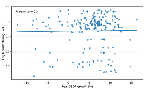
Figure 3. Relationship between GSDP Growth and Manufacturing GVA

Note: Each point represents a state-year observation. The fitted line shows the unconditional linear trend. (Sample : 196 state-year observations)

Comparative and Within-state Descriptive Analysis

The pooled correlations provide a useful first indication of the direction and strength of the relationships, but panel data also permit a within-state perspective. The within-state correlations are calculated after removing each state’s own mean from the variables. They therefore ask whether deviations above a state’s usual level of the explanatory variable are associated with deviations above its usual level of manufacturing GVA. These statistics remain descriptive and are not causal estimates.

Table 4: Pooled and within-state correlations

Variable	Pooled correlation with log Manufacturing GVA	Within-state correlation
State Tax Effort	0.484	0.408
Credit/GSDP	0.561	0.356
GSDP growth	0.014	0.291

Source: Author’s calculation based on secondary data

Note: Within-state correlations are based on deviations from state-specific means. They are presented as descriptive statistics and should not be interpreted as causal effects.

Overall, the variable-wise analysis shows that tax burden and Credit/GSDP are positively associated with manufacturing GVA in the pooled data, whereas GSDP growth has virtually no pooled contemporaneous correlation with the dependent variable. The positive within-state correlations suggest that these relationships are not solely attributable to permanent differences between states. However, the descriptive results cannot isolate the effect of tax burden from other factors or common shocks. This motivates the use of a two-way fixed-effects specification in the next section.

5. Econometric Results

The descriptive analysis indicates positive raw associations between tax burden, credit availability and manufacturing GVA, but these associations may reflect persistent differences across states and common time shocks. Section 4 therefore estimates a two-way fixed-effects panel model to examine whether the relationship between tax burden and manufacturing performance remains after accounting for state-specific and year-specific effects and the included control variables.

Empirical Model:

ln(MFGVAᵢₜ) = αᵢ + λₜ + β₁ State Tax Effortᵢₜ + β₂ GSDPGrowthᵢₜ + β₃ Credit/GSDPᵢₜ + εᵢₜ

Here, i denotes the state and t denotes the year. αᵢ represents state fixed effects, which absorb time-invariant differences across states such as geography, historical industrial structure and other persistent characteristics, λₜ represents year fixed effects, which absorb shocks common to all states in a given year. The model uses log manufacturing GVA as the dependent variable and includes tax burden as the main explanatory variable, with real GSDP growth and Credit/GSDP as controls. For coefficient interpretation, tax burden is entered as a proportion (e.g., 0.10 = 10%), while real GSDP growth and Credit/GSDP are expressed in percentage-point units in the baseline regression specification.

Baseline Fixed-Effects Results

Table 5 : Baseline Two-Way Fixed-Effects Estimates

Variable	Coefficient	Std. Error	p-value
State Tax Effort	0.910	2.364	0.703
GSDP growth	0.005	0.005	0.336
Credit/GSDP	0.002	0.004	0.588
State fixed effects	Yes	—	—
Year fixed effects	Yes	—	—
Observations	196	—	—

Source: Author’s calculation based on secondary data

Note: Standard errors and p-values are reported as provided by the project baseline estimation output. No additional claim is made here about the covariance estimator beyond the source output.

Interpretation of the Baseline Estimates

State Tax Effort – The coefficient on tax burden is positive (0.910). Because tax burden is entered as a proportion, a one-percentage-point increase in tax burden corresponds to an approximate 0.91% increase in manufacturing GVA, holding the other included variables and fixed effects constant. However, the estimate is statistically insignificant (p = 0.703), so the baseline model does not provide statistically reliable evidence of a non-zero association between tax burden and manufacturing GVA.

GSDP growth – The coefficient on real GSDP growth is positive (0.005). Since the variable is expressed in percentage points, a one-percentage-point increase in GSDP growth is associated with an approximate 0.50% increase in manufacturing GVA, ceteris paribus. The estimate is statistically insignificant (p = 0.336), and therefore the model does not provide sufficient evidence of an independent statistically significant relationship in the baseline specification.

Credit/GSDP – The coefficient on Credit/GSDP is positive (0.002). With Credit/GSDP expressed in percentage-point units in the baseline regression, a one-percentage-point increase is associated with an approximate 0.20% increase in manufacturing GVA, holding other factors constant. This coefficient is also statistically insignificant (p = 0.588). Thus, after controlling for the fixed effects and the other explanatory variables, the baseline model does not identify a statistically significant independent association between credit availability and manufacturing GVA.

Overall statistical significance – All three p-values exceed 0.10: 0.703 for tax burden, 0.336 for GSDP growth, and 0.588 for Credit/GSDP. Accordingly, none of the explanatory variables is statistically significant even at the 10% level. The positive signs of the coefficients should therefore not be interpreted as evidence of statistically established positive effects.

6. Visual Summary: Coefficient Estimates with 95% Confidence Intervals

Figure 4 presents the estimated percentage change in manufacturing GVA associated with a one-percentage-point increase in each explanatory variable, together with the corresponding 95% confidence interval. The figure 4 provides a visual summary of both the direction and statistical uncertainty of the baseline estimates.

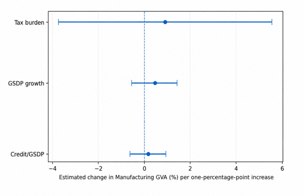
Figure 4: Estimated Change in Manufacturing GVA (%) per One-percentage-point Increase, with 95% Confidence Intervals

Note: Tax burden is entered as a proportion, whereas GSDP growth and Credit/GSDP are expressed in percentage-point units. The 95% confidence intervals are calculated using the standard errors reported in the baseline estimation output.

The 95% confidence interval for tax burden is approximately -3.72% to 5.54%; for GSDP growth it is approximately -0.48% to 1.48%; and for Credit/GSDP it is approximately -0.58% to 0.98%. In every case, the interval crosses zero. This indicates that the data are consistent with a zero effect as well as with positive or negative values within the respective interval, which is consistent with the statistical insignificance of all three coefficients.

Interim Summary – Taken together, the baseline two-way fixed-effects results do not provide statistically significant evidence that state-level tax burden is associated with manufacturing GVA over the study period. Although the tax-burden coefficient is positive, its p-value is well above conventional significance thresholds. The coefficients on GSDP growth and Credit/GSDP are likewise positive but statistically insignificant. The contrast between the moderate positive raw correlation of tax burden with manufacturing GVA (r = 0.484) and the statistically insignificant fixed-effects coefficient indicates that the unconditional association should not be interpreted as a causal effect. These baseline results should be considered alongside the diagnostic and robustness checks in Section 7 and key findings section.

To robustness, the connection between tax burden and manufacturing GVA is investigated under three different model formulations. There are no statistically significant evidence of an association between tax burden and manufacturing GVA in the baseline fixed-effects model, which produces a tax coefficient of 0.910 p = 0.703, n = 196.The estimated tax coefficient increases numerically to 3.929 in the lagged-tax specification, but remains statistically insignificant (p = 0.441). This is a difference of more than three points from the baseline. Although the coefficient is still statistically insignificant at conventional levels, this trend is consistent with a greater connection when lagged effects are taken into consideration. The coefficient drops to 0.713 p = 0.707, n = 140, closer to the baseline value, when COVID-affected observations are excluded No COVID model. The smaller sample size 140 vs. 196 observations should be taken into account when evaluating this comparison, this is consistent with the COVID period not being the main driver of the tax-manufacturing link seen in the lagged specification. The tax coefficient, which ranges from 0.713 to 3.929, is statistically negligible across all three specifications p > 0.44 in every instance. The positive sign of the tax-burden coefficient is preserved across the alternative specifications, although its magnitude varies and none of the estimates is statistically significant.

7. Diagnostic and Robustness Checks

Two alternative models were used to examine the link between tax burden and manufacturing Gross Value Added (GVA) in order to test the stability of the baseline fixed-effects (FE) estimations.

The following table provides the details of the alternative models.

Table 6 : Alternate Models

Model	State_Tax_Effect	P_value	Observations
Baseline FE	0.91	0.703	196
Lagged Tax	3.929	0.441	168
No COVID	0.713	0.707	140

Lagged Tax Model

A lagged specification was provided to partially address potential reverse causality and to account for the likelihood that changes in tax policy take time to affect industrial performance. This model uses the following formula to substitute a one-year lag State Tax Effort_i,t-1 for the contemporaneous tax variable:

ln(MFGVAᵢₜ) = α_i + λ_t + β₀ + β₁ State Tax Effortᵢ,ₜ_-1 + β₂ GSDPGrowthᵢₜ + β₃ Credit/GSDPᵢₜ + εᵢₜ

Where:

•  i denotes the individual state, and t denotes the financial year.
• ln(MFGVAᵢₜ) is the natural logarithm of real Manufacturing Gross Value Added, which serves as the dependent variable measuring manufacturing performance.
• β₀ is the intercept (or constant term) of the regression model.
•  β₁ is the primary coefficient of interest. It estimates the association between the state tax effort—measured as a one-year lag (State Tax Effort_i,t-1) and manufacturing GVA.
• β₂ and β₃ are the coefficients for the control variables, capturing the effects of real GSDP growth  and credit availability, respectively.
• α_i  represents the state fixed effects, which account for unobserved, time-invariant characteristics specific to each state, such as geography, long-run policy environments, or historical industrial structures.
• λ_t represents the year fixed effects, which absorb common macroeconomic shocks or nationwide policy changes affecting all states simultaneously in a given year.
• εᵢₜ is the idiosyncratic error term.

The sample size drops from 196 to 168 observations because of the one-year lag. In comparison to the baseline estimate of 0.910, the predicted tax coefficient in this model increases numerically to 3.929. The coefficient is still statistically insignificant at conventional levels, according to the p-value of 0.441, despite this numerical increase.

No COVID Model

A secondary robustness check was carried out by removing the years affected by the COVID-19 pandemic to make sure the baseline results were not disproportionately influenced by the severe economic disruptions caused by the epidemic. The model was recalculated with the precise requirement that time t≠ 2020, 2021:

ln(MFGVAᵢₜ) = α_i + λ_t + β₀ + β₁ State Tax Effortᵢₜ + β₂ GSDPGrowthᵢₜ + β₃ Credit/GSDPᵢₜ + εᵢₜ

Where:

• i denotes the individual state, and t denotes the financial year. Crucially for this model, the financial years 2020-21 and 2021-22 are excluded (t ≠2020,2021) to remove the economic distortions caused by the pandemic.
• ln(MFGVAᵢₜ) is the natural logarithm of real Manufacturing Gross Value Added for state  in year .
• β₀ is the intercept (or constant term) of the regression model.
• β₁ is the primary coefficient of interest, estimating the contemporaneous association between the state tax effort and manufacturing GVA.
• β₂ and β₃ are the coefficients for the control variables, capturing the effects of real GSDP growth and credit availability, respectively.
• α_i represents the state fixed effects, which account for unobserved, time-invariant characteristics specific to each state. 
• λ_t  represents the year fixed effects, which absorb common macroeconomic shocks affecting all states in the remaining non-COVID years.
• εᵢₜ is the idiosyncratic error term.

The number of observations decreases to 140 when these years are excluded. The tax coefficient is estimated at 0.713 with this specification, which is nearer the baseline value. This coefficient’s p-value of 0.707 indicates that even when abnormal economic eras are eliminated from the sample, the association is still statistically insignificant.

The tax variable’s coefficient continuously maintains a positive sign in all assessed models Baseline FE, Lagged Tax, and No COVID but it is not statistically significant. Throughout the requirements, the p-values vary from 0.441 to 0.707. The baseline conclusion that there is not enough statistical evidence to demonstrate a meaningful correlation between state tax effort and manufacturing GVA over the research period is confirmed by these alternative models.

KEY FINDINGS

This section draws together the qualitative insights emerging from the literature review and the design of the empirical model, ahead of formal estimation. Rather than reporting numerical coefficients, it summarises the substantive patterns, tensions and expectations that motivate the study and that will guide interpretation once the regression is estimated.

1. A slow but Incomplete Shift Toward Tax Simplification

The literature consistently explains about India’s tax system as having shifted from from a complex, decimated structure toward one that is simpler, more transparent and more predictable, particularly through the introduction of GST. This shift is treated across multiple studies as a positive step for the business environment. However, the literature does not treat this shift as complete — several authors continue to flag complexity, compliance burden and uncertainty as live concerns even after GST, suggesting that simplification has been a direction of travel rather than a resolved outcome. This supports the choice of using the post-GST period (FY 2017–18 onward) as the empirical window, since it captures the period during which this shift was expected to have its clearest effect on manufacturing.

2. Tax Burden Is Widely Assumed to Matter, but Rarely Measured Empirically

Across the literature, taxation is treated as an important influence on investment and business decisions, and high or uncertain effective tax rates are repeatedly linked to weaker investor confidence. However, most of this evidence is descriptive or policy-based rather than measured statistically. Only a small number of studies — notably Hussain (2023) and Sankarganesh and Shanmugam (2023) — offer econometric evidence, and both are confined to a single reform episode, the 2019–20 corporate tax cut. This points to a genuine gap: the broader, ongoing relationship between state-level tax burden and manufacturing performance over time has not been systematically tested. The present study’s panel design, covering 28 states across seven years, is intended to address this gap by examining the relationship as an ongoing pattern rather than a single before-and-after comparison.

3. A Gap Between Investment Climate and Manufacturing Performance

A recurring and important tension in the literature is that improvements in the investment climate do not appear to translate automatically into stronger manufacturing outcomes. Som (2018) finds that manufacturing value added remained largely stagnant relative to GDP even as FDI inflows and investor sentiment improved. This is reinforced by Deodhar (2015) and Kadekodi (2018), who argue that structural constraints — infrastructure, land acquisition, labour regulation, and access to skilled labour and finance — continue to limit how much manufacturing can respond to a more favourable tax and investment environment. This suggests that even if the empirical model finds a meaningful association between tax burden and manufacturing GVA, this relationship is likely to be one contributing factor among several, rather than a complete explanation of manufacturing performance across states.

4. Financing Conditions and Broader Growth Are Likely Confounding Factors

The inclusion of GSDP growth and Credit/GSDP as control variables reflects a recurring theme in the literature: manufacturing performance is shaped jointly by taxation, general economic conditions and access to finance, and these factors tend to move together. Without controlling for these, an observed relationship between tax burden and manufacturing performance could partly reflect broader economic cycles or credit availability rather than tax policy itself. This reinforces the importance of the fixed-effects design and control variables specified in Section 5 for isolating the tax–manufacturing relationship as far as possible with observational, state-level data.

5. Implications for the Research Gap

Taken together, these qualitative patterns suggest that the relationship between tax reform and manufacturing performance under Make in India is unlikely to be straightforward. The literature supports the expectation that a lower or more stable tax burden is generally associated with a more favourable investment climate, but it also cautions that this improved climate has not clearly shown up in manufacturing value added at the higher level. The present study is positioned to clarify part of this puzzle by testing whether the relationship holds at the state level using a longer, systematic panel, rather than relying on a single reform episode or aggregate national trends.

DISCUSSION

The empirical findings indicate that state Tax Effort is positively related to manufacturing GVA in the descriptive analysis, but the estimated relationship is not statistically significant once state and year fixed effects and the selected control variables are taken into account. The baseline coefficient of 0.910, with a p-value of 0.703, therefore does not provide sufficient statistical evidence of a significant association between state Tax Effort and manufacturing performance. The result suggests that differences in own-source revenue mobilisation, considered on its own, do not explain the observed variation in manufacturing performance across the states in the sample. The contrast between the descriptive and fixed-effects results is important for interpretation.

The descriptive association may reflect persistent differences across states or changes over time that are not captured when the variables are considered without controls. Once state-specific characteristics and common year effects are accounted for, the relationship between state Tax Effort and manufacturing performance becomes statistically insignificant. This indicates that manufacturing outcomes are likely shaped by a wider set of economic and institutional conditions rather than by state tax effort alone. The robustness results support the same interpretation. The relationship remains statistically insignificant when state Tax Effort is introduced with a lag and when the COVID-19 period is excluded from the analysis. These specifications do not materially change the inference from the baseline model, suggesting that the main finding is not driven solely by the timing of state tax effort or by the unusual conditions associated with the pandemic period.

The findings should not be interpreted as showing that taxation is irrelevant to manufacturing. Rather, within the present sample and model, there is insufficient statistical evidence that higher state Tax Effort by itself is associated with better manufacturing performance after accounting for state and year effects, overall economic growth, and credit availability. This points to the importance of considering other conditions, including infrastructure, finance, skills, technology, and related policy factors, when assessing manufacturing performance. Make in India provides the broader policy context for the study, but the analysis does not estimate its causal effect.

CONCLUSION

In this paper, we examined the relationship between state Tax Effort and manufacturing performance in India during the post-GST period using data from 28 states for the period FY 2017–18 to FY 2023–24. Our descriptive analysis reveals a positive association between state Tax Effort and manufacturing GVA. However, this association is no longer statistically significant after controlling for state and year fixed effects and other covariates. Consequently, we find insufficient statistical evidence of a significant association between state Tax Effort and manufacturing performance in the post-GST period.

Our findings highlight the complexity of the determinants of manufacturing performance. Manufacturing performance is influenced by a range of factors, and taxation in isolation may not be a determining factor. The difference between the descriptive association and the fixed-effects results suggests that the observed descriptive association may reflect differences across states and over time in other determinants of manufacturing performance that are not fully captured by the model.

Future research could build on our analysis by extending the period of analysis and employing richer datasets. Researchers may also consider examining alternative measures of state Tax Effort and manufacturing performance and exploring whether the association between these variables differs across specific dimensions.

Finally, we view Make in India as the overarching policy framework within which the post-GST developments and manufacturing performance more generally need to be understood. However, we do not attempt to evaluate the causal effect of the Make in India initiative itself. Future research may adopt a broader perspective in understanding manufacturing performance by complementing the analysis of taxation with an examination of other factors and policies that shape the manufacturing sector. Infrastructure, finance, skills, and related reforms are important potential determinants of manufacturing performance in India, and future research may build on the analysis in this paper to explore their relationships with manufacturing performance in greater detail.

REFERENCES

Bala, M. (2018). GST in India and its impact on the Indian economy. Paper presented at the One Day National Seminar on “GST – Impact on Indian Economy,” Hindu Girls College, Jagadhari, Haryana, India.

Deodhar, S. Y. (2015). Make in India: Re-chanting the mantra with a difference (W.P. No. 2015-02-02). Indian Institute of Management Ahmedabad.

Hussain, A. (2023). Effect of tax cut on investment: Evidence from Indian manufacturing firms (NIPFP Working Paper No. 390). National Institute of Public Finance and Policy.

Kadekodi, G. K. (2018). Make in India: Policy drives and challenges. In V. B. Annigeri, R. S. Deshpande, & R. Dholakia (Eds.), Issues in Indian public policies (pp. 83–105). Springer. https://doi.org/10.1007/978-981-10-7950-4_4

Moid, S. (2017). The challenge of reforming the Indian tax system for enabling Make in India. FIIB Business Review, 6(3), 12–17.

Ojha, R., & Vrat, P. (2019). Implications of Goods and Services Tax reform on the Make in India initiative: A system dynamics perspective. Systems Research and Behavioral Science, 36(4), 551–563. https://doi.org/10.1002/sres.2570

Prasath, V. L. (2026). Impact of goods and service tax with the recent scenario in India. International Journal for Multidisciplinary Research.

Rao, M. G., & Kumar, S. (2018). Envisioning tax policy for accelerated development in India (Working Paper No. 17/190). National Institute of Public Finance and Policy.

Rao, M. G., & Rao, R. K. (2009). Tax system reform in India. Initiative for Policy Dialogue Working Paper Series.

Singh, R. R. (2016). Improving taxation environment: Attracting foreign direct investment (Working Paper No. 325). Indian Council for Research on International Economic Relations.

Sankarganesh, K., & Shanmugam, K. R. (2023). Effect of corporate income tax on investment decisions of Indian manufacturing firms. Journal of the Asia Pacific Economy, 28(1), 156–175. https://doi.org/10.1080/13547860.2021.1873896

Thomas, A., Joumard, I., Hanappi, T., & Harding, M. (2017). Taxation and investment in India. OECD.

Tripathy, A., & Dastrala, S. M. (2023). Make in India: So far and going ahead (IIMB Working Paper No. 674). Indian Institute of Management Bangalore.

Kadekodi, G. K. (2017). Make in India: Policy drives and challenges.

Reserve Bank of India. (2023). State Finances: A Study of Budgets of 2023–24: Revenue Dynamics and Fiscal Capacity of Indian States. RBI.

Reserve Bank of India. (2023). Handbook of Statistics on Indian States 2022–23. RBI.

Reserve Bank of India. (2023). Annual Report 2022–23. RBI.

Ghosh, S., et al. (2021). Local banking and manufacturing growth: Evidence from India. IIMB Management Review, 33(2), 95–104.

Shukla, S., & Singh, R. (2018). GST in India: Performance of companies after one-year of roll out. Indian Journal of Finance, 12(11), 37–48.